
供應 65K MAC 的記憶體階層:TPU v1 的資料壽命與重用
TPU v1 的記憶體階層依資料壽命、重用方式與數值寬度分工,讓較慢的外部供應支撐較快的片上運算。這個設計不會消除 memory wall;它把成功條件轉成 tile 是否重用、weights 能否及時到位,以及 partial sums 是否留在適當層級。
INT8 降低算術成本後,65,536 個 MAC 需要規律供料。公開架構中的 activation path 約為 167 GiB/s,外部 weight DDR3 則約為 30 GiB/s;這兩條路徑承載不同資料,不能直接拿頻寬差距當成利用率。必須先看哪些資料從外部取得、能在片上重用多久,以及每個運算階段的消費速率。Google TPU v1 deep dive
因此,理解加速器的儲存容量,還要理解排程與 live state。以下把 weights、activations 與 partial sums 分開追蹤,推導 Unified Buffer、Weight FIFO 及 Accumulator 的角色,再分析什麼 shape 或 batch 會使陣列等待。這能用來判斷新增 SRAM、頻寬或 MAC,哪一項才會改善目標工作負載。
先依圖把三類資料分開:weights 從外部記憶體進入,activations 在片上 buffer 供應,partial sums 留在累加路徑。這些箭頭不是同一種頻寬;資料可以在哪裡停留、重用幾次,才會決定外部供應能否支撐陣列。
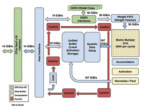
一塊 memory 無法同時滿足三種資料
神經網路 inference 的三種主要狀態,存取行為完全不同。
Weights 很大,但推論期間基本上只讀;同一組 weights 可以服務一批 input。Activations 與 layer intermediate 的容量小得多,卻會在相鄰 layers 之間反覆讀寫。Partial sums 更特殊:每個 dot product 會把大量窄乘積累加成較寬的數值,寫入頻率高,而且不能跟 input 一樣維持 8-bit。
TPU v1 因此把資料拆成三個層級:
- 8 GiB off-chip DDR3 Weight Memory:保存大量 read-only model weights。
- 24 MiB on-chip Unified Buffer:保存 activations 與 intermediate results,直接作為 Matrix Unit input。
- 4 MiB 32-bit Accumulators:保存 Matrix Unit 產生的 partial sums。
Weights 到 Matrix Unit 中間再加一層 Weight FIFO;Matrix Unit 本身保留一個 64 KiB weight tile,並有另一份 tile 做 double buffering。論文指出 Weight FIFO 深度為四個 tiles,目的在於讓 weight fetch 與 execution 解耦。ISCA 2017 PDF
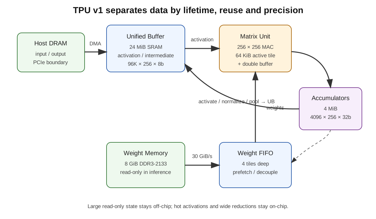
這種切割的價值,在於每一塊 memory 都只為一類問題付成本。若把 8 GiB weights 全做成 on-chip SRAM,die area 不可能接受;若把 activations 留在 DDR3,167 GiB/s 的 Matrix Unit input rate根本供不上;若 partial sum 也壓成 INT8,幾百個 products 累加後很快 overflow。
memory hierarchy 因此不是附屬於 compute 的配角。它其實在回答:哪些 bytes 值得留在最昂貴的 on-chip area,哪些可以接受 off-chip latency,哪些必須用更寬 precision 保存。
24 MiB Unified Buffer 比 cache 更接近軟體管理的 register file
Google 把 Unified Buffer 描述成 24 MiB SRAM;Google Cloud 的介紹甚至用「work as registers」來形容它。Google Cloud
它和 CPU cache 最大的差異,不只是容量。
Cache 需要 tag、replacement policy、miss handling、coherence 或至少 cache-management machinery,硬體會動態猜哪些資料應該留下。TPU v1 的 Unified Buffer 更接近 software-managed scratchpad:compiler/runtime 明確安排資料何時從 host 搬進來、哪一塊 address range 保存哪個 activation、何時再送進 Matrix Unit。
24 MiB 可以寫成:
96K × 256 × 8 bit = 24 MiB
每一列剛好是 256 個 INT8 element,也就是 Matrix Unit 每 cycle 的 activation width。另一個直觀換算是:
24 MiB / 64 KiB = 384
如果只用最簡化的 256×256 INT8 activation tile 來看,Unified Buffer 理論上可以容納 384 個 64 KiB tiles。真實 compiler allocation 還會受到 tensor shape、padding、不同 layer 的 live range 與 input/output overlap 影響,但這個量級已足以看出它不是一般小型 cache。
更重要的是頻寬。256 bytes/cycle 在 700 MHz 下就是約 167 GiB/s。這條 on-chip path 比 30 GiB/s 的 weight DDR3 高約 5.6 倍,比 host PCIe effective bandwidth 更高一個數量級。
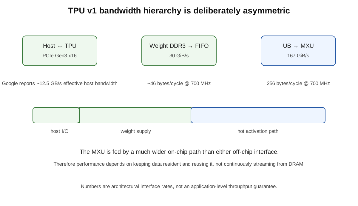
這種 scratchpad 設計的 trade-off 很明確。硬體變得簡單、資料位置可預測,P99 latency 也比較不會受到 cache miss pattern 擾動;代價則是 compiler 必須自己管理 live range、搬移與 overlap。cache 把複雜度放在 silicon;TPU v1 把相當一部分複雜度推回 compiler。
論文還透露一個很實際的 physical-design 決策:24 MiB 的大小部分原因是配合 Matrix Unit 在 die 上的 pitch,同時在極短開發週期下讓 compiler 更容易處理。floorplan 裡 Unified Buffer 約佔 29% die、Matrix Multiply Unit 約 24%、Accumulators 約 6%;control 僅約 2%。Jouppi et al., ISCA 2017
這提醒我們 accelerator architecture 並不是把抽象模型最佳化到極致。SRAM 容量、macro shape、wire pitch、compiler complexity 與 time-to-deploy 會一起決定最後的數字。
Weight FIFO 解的是等待時間,重用才解得了頻寬
Weight path 更容易被誤解。
TPU v1 的 weights 放在 8 GiB DDR3 Weight Memory,推論期間是 read-only。這讓一張卡可以同時保存許多 production models,不需要每次 inference 都從 host PCIe 重傳整個模型。真正計算前,weights 先被讀進 on-chip Weight FIFO,再送到 Matrix Unit。
Matrix Unit 的一個 weight tile 是:
256 × 256 × 8 bit = 64 KiB
論文指出,把這個 tile shift 進 systolic array 需要 256 cycles,所以 Matrix Unit 放了第二份 tile 做 double buffering;當 tile A 正在計算,tile B 可以準備進入下一輪。Weight FIFO 又再往前放四個 tiles,讓 Read_Weights 採用 decoupled access/execute:送出 address 之後,不必等整個 fetch 完成才讓 instruction 本身結束。若 activation 或 weights 還沒 ready,Matrix Unit 才會真正 stall。Jouppi et al., ISCA 2017
但 FIFO 只能藏 latency,不能違反 bandwidth conservation。
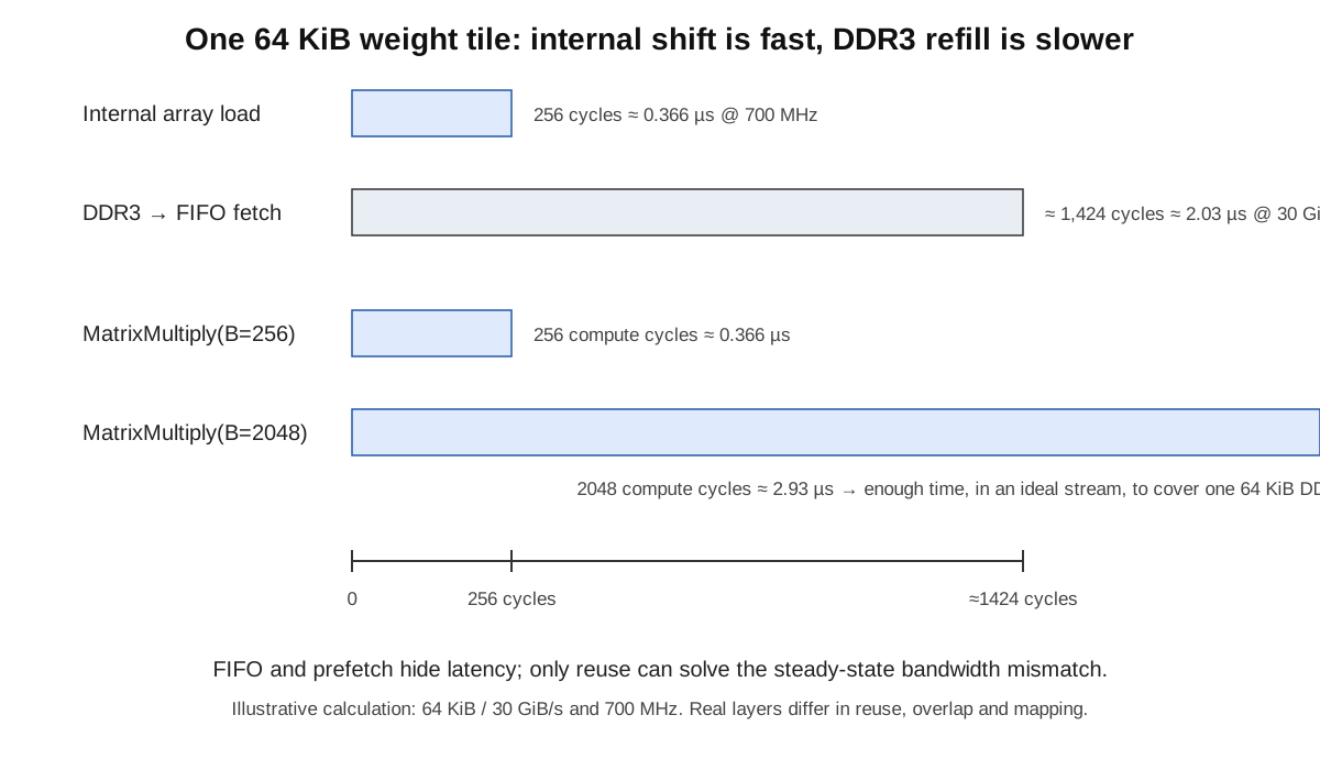
用公開數字做一個理想化算例。64 KiB weight tile 從 30 GiB/s DDR3 搬進來,單純 serialization time 約:
64 KiB / 30 GiB/s ≈ 2.03 µs
700 MHz 下約是:
2.03 µs × 700 MHz ≈ 1,424 cycles
相較之下,tile 從 Matrix Unit 的內部 buffer 以 256 bytes/cycle shift 進 256×256 array,只需要:
64 KiB / 256 B = 256 cycles ≈ 0.366 µs
這兩個數字不是矛盾;它們是兩個不同階段。外部 DDR3 → Weight FIFO 是較慢的 refill path,FIFO / local buffer → array 是較寬的內部 path。
現在把它和 systolic-array 那篇的 MatrixMultiply(B) 接起來。
若同一個 256×256 weight tile 只處理 B=256 rows,compute window 約 256 cycles,也就是 0.366 µs。外部 DDR3 fetch 一份新 tile 卻要約 1,424 cycles。就算 FIFO 已經提前抓資料,長期 steady state 還是不能每 256 cycles 消耗一個全新的 tile,因為上游每秒供應的 bytes 不夠。
如果 B=2048,同一組 weights 被 2048 rows 重用,compute window 約 2.93 µs;在理想連續傳輸下,已經長於一個 64 KiB tile 的 2.03 µs DDR3 fetch。這時 weight bandwidth 比較有機會被藏在計算後面。
這個算例刻意簡化,不能當成 TPU layer 的實測 performance。真實模型還有多個 tiles、不同 shapes、pipeline overlap、DDR bank behavior 與 compiler scheduling。但它揭露了最重要的關係:
FIFO 解 latency;data reuse 解 bandwidth。
如果 arithmetic intensity 不夠,再深的 FIFO 最後還是會空。
4 MiB Accumulator 是 reduction state,不是一般 activation storage
另一個容易被忽略的元件是 4 MiB Accumulator memory。
INT8 × INT8 會產生較寬 product,而一個 dot product 還要把數百個 product 相加。前一篇已用 worst-case 算例說明,256 個 127×127 累加後 magnitude 已接近 22 bits;因此 TPU v1 用 32-bit accumulator 保存 partial sums。
4 MiB 的組織是:
4096 × 256 × 32 bit = 4 MiB
256 對應 Matrix Unit 每 cycle 輸出的 256 個 partial sums;4096 則不是任意數字。論文說明,TPU roofline 的 knee 大約需要 1350 operations/byte 才能到 peak,設計先把 accumulator depth round 到 2048,再複製一份讓 compiler 可以 double buffer,最後得到 4096 rows。Jouppi et al., ISCA 2017
這裡可以看到一個很漂亮的 cross-layer loop:
external memory bandwidth → roofline knee → required reuse window → accumulator capacity → compiler double buffering
也就是說,Accumulator 容量不是只由「一個 tensor 多大」決定,而是被整顆晶片要維持 peak throughput 所需的 arithmetic intensity 反推回來。
當 Matrix Unit 完成 accumulation,資料再經 activation、normalize / pool 等 pipeline,最後寫回 Unified Buffer,成為下一層的 input。這讓 intermediate result 大多數時間留在 chip 上,不必每個 layer 都穿過 PCIe 或 DDR3。
Failure mode 很單純:資料沒到,65K MAC 一起等
TPU v1 沒有複雜 cache miss hierarchy,並不代表 memory stall 消失。相反地,stall 的原因被變得更直接。
論文描述 Matrix Unit 的原則就是 keep it busy;如果 input activation 或 weight data 沒 ready,Matrix Unit 會 stall。Weight load 可以 decoupled 發出、activation 可以由 compiler 提前搬到 Unified Buffer,但任何一段 schedule 算錯,最後都會在同一個地方付代價:整個 256×256 array 沒有有效 work。
可以想像一個 failure scenario:
- compiler 預期 tile N+1 已透過
Read_Weights進入 FIFO; - DDR3 service time 因前面 traffic 或 mapping 比估計更久;
- tile N 計算結束;
- next tile 尚未 ready;
- Matrix Unit stall,65,536 個 MAC 同時閒置。
這和 CPU cache miss 的表面症狀不同,但本質一樣:compute pipeline 等 memory。TPU 的優勢是 state 比較顯式、可預測;劣勢是 compiler/runtime 必須更準確地把資料搬移排進 timeline。
因此 software-managed memory 不會免費得到 deterministic performance。它只是把「硬體動態猜測」換成「軟體靜態安排」。當 workload shape 很規律,這筆交換非常划算;當 shape、sparsity 或 control flow 變得高度動態,compiler burden 就會急速上升。
為什麼六個 production workload 裡四個仍然 memory-bound
第一代 TPU 已經做了很多看似極端的 data-movement optimization:
- INT8 把 operand bytes 壓小;
- systolic array 讓資料在鄰近 MAC 間重用;
- 24 MiB Unified Buffer 把 hot activation 留在片上;
- Weight FIFO 與 double buffering 提前搬 weights;
- 4 MiB Accumulator 讓 reduction 不必反覆寫回外部 memory。
結果仍然是 Google 報告六個代表性 workload 中有四個落在 memory-bound 區域;論文甚至估計,如果把 TPU weight memory 換成當時 K80 等級的 GDDR5,achieved TOPS 可以接近三倍。Jouppi et al., ISCA 2017
這不表示 TPU v1 的 memory hierarchy 設計失敗。剛好相反:它把 arithmetic 成本壓低到足以讓下一個限制清楚浮現。
CNN 的 convolution 通常能讓 weights 在大量 spatial positions 上反覆使用,因此 arithmetic intensity 高,比較容易靠近 compute roof。Fully connected 與 LSTM layer 的 weight reuse 較低,大量參數必須持續從 weight memory 送進來,就更容易撞到 30 GiB/s 的斜率上限。下一階段真正要分析的,就是 operations/byte 如何決定同一顆 TPU 到底看到 92 TOPS,還是只看到一小部分。
不過在進入 roofline 之前,還有一個 production constraint 不能跳過。
提高 B 可以增加 weight reuse、比較容易把 30 GiB/s fetch 藏在計算後面;但線上 inference 的 request 不能無限等 batch。當服務要求 P99 latency,例如 TPU v1 論文中 MLP0 約 7 ms 的 tail-latency constraint,硬體利用率與 batch size 就會直接衝突。
所以 memory hierarchy 最後把問題推到下一層:資料重用需要時間,線上服務卻限制你能等多久。
下一篇會處理 TPU v1 的 #05:P99 latency 與 throughput 為什麼會迫使 datacenter inference processor 採用和傳統 throughput machine 不同的設計。